Chapter 5 : Dynamic performance analysis tools

5.1. Dynamic performance

1) Give the 5% settling time, the rise time from 5% to 95% and the peak time.

Actuator 1 : $t_s\approx 1.1\, s$, $t_r \approx 0.1\, s$, $t_p\approx 0.25\, s$.
Actuator 2 : $t_s\approx 0.38\, s$, $t_r \approx 0.35\, s$, there are no oscillations.
Actuator 3 : $t_s\approx 1.5\, s$, $t_r \approx 1.4\, s$, there are no oscillations.

2) Give the first overshoot and the period of pseudo-oscillations.

Actuator 1 : $M_p\approx 50\%$, $T \approx 0.5\, s$.
Actuator 2 and Actuator 3 : there are no oscillations.

3) Calculate the gain corresponding to this specific frequency, in decimal units and in decibels.

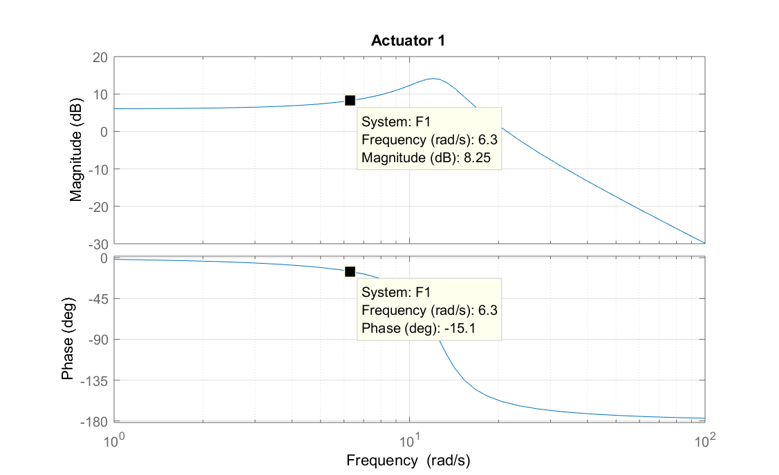
Actuator 1 : $G(6.3)\approx 2.5\approx 8\, dB$.
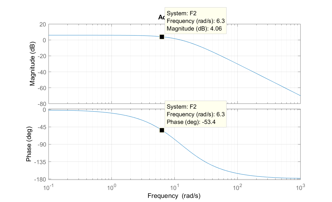
Actuator 2 : $G(6.3)\approx 1.6\approx 4\, dB$.
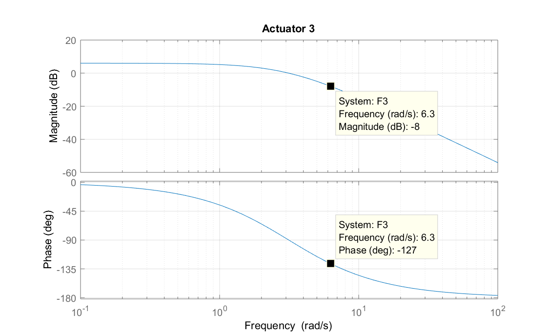
Actuator 3 : $G(6.3)\approx 0.4\approx -8\, dB$.

4) Calculate the phase shift corresponding to this specific frequency, in degrees.

Actuator 1 : $\Delta t \approx 0.04\, s \Rightarrow \varphi(6.3)\approx -14°$.
Actuator 2 : $\Delta t \approx 0.15\, s \Rightarrow \varphi(6.3)\approx -54°$.
Actuator 3 : $\Delta t \approx 0.35\, s \Rightarrow \varphi(6.3)\approx -126°$.

5) On the Bode diagrams corresponding to the three actuators (cf. figure 5.34), indicate the points that correspond to the tests illustrated in figure 5.33. Verify the consistency of the previously calculated gains and phase shifts with those resulting from the Bode diagrams.

6) On the Bode diagrams find the cut-off frequencies at -3 dB.

Actuator 1 : $\omega_c\approx 19 \, rad/sec$
Actuator 2 : $\omega_c\approx 8 \, rad/sec$
Actuator 3 : $\omega_c\approx 2 \, rad/sec$

7) On the Bode diagrams find the resonance frequencies and the quality (resonance) factor, $Q$.

Only actuator 1 has resonance, for which $\omega_r\approx 12\, rad/sec$ and $Q\approx 8\, dB$.

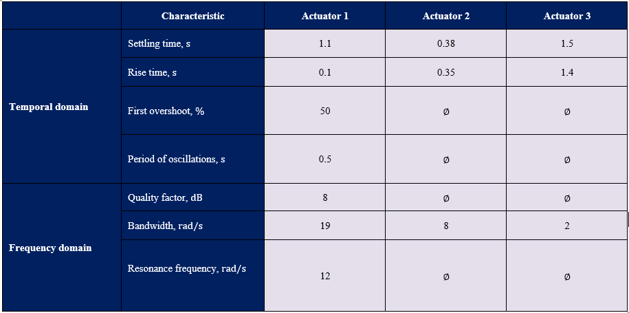
8) Fill in the table 5.7 the values of the previously identified performance indicators and highlight the existence of qualitative relations between the indicators in the temporal domain and the indicators in the frequency domain.

5.2. Transfer functions

1) Write the dynamic equation of the motion of the object for the two configurations. The position of the mass is denoted by $x$ and for each configuration the positive direction is taken as indicated in figure 5.36.b and c. For each configuration, the origin of the system of coordinates is located on the electromagnet.

For the repulsive force: $m\ddot{x}=c\frac{i^2}{x^2}-mg$

For the attractive force: $m\ddot{x}=mg-c\frac{i^2}{x^2}$

2) Explain why this system of input $i$ and output $x$ is nonlinear.

The square on the current and the position, the division between these two and the sum with a constant are nonlinear functions.

3) For the two configurations, determine the position of equilibrium $x_{eq}$ for a rated hold current in the magnet of $20 \, A$, if the coefficient $c=0.027\, Nm^2A^{-2}$.

For both cases $x_{eq}=1\, cm$

4) The focus is now on vertical motions of the mass around its equilibrium position $x_{eq}$. Show that the linearization of the system around the equilibrium ($i_{eq},\, x_{eq}$) gives the differential equation $\ddot{\Delta x}=\alpha\Delta i+\beta\Delta x$ where $\Delta i$ is the current variation around the rated hold current $i_{eq}$ and $\Delta x$ is the variation of the position of the object around $x_{eq}$. Find the analytical expressions of $\alpha$ and $\beta$ for these two configurations.

For the repulsive force : $\alpha=2\frac{mg}{i_{eq}}\quad\text{and}\quad \beta=-2\frac{mg}{x_{eq}}$

For the attractive force : $\alpha=-2\frac{mg}{i_{eq}}\quad\text{and}\quad \beta=2\frac{mg}{x_{eq}}$

5) $\Delta I(s)$ and $\Delta X(s)$ denote the Laplace transforms of $\Delta i$ and $\Delta x$, respectively. Calculate the transfer function $H(s)$ of the linearized system around the equilibrium position.

$$H(s)=\frac{\alpha}{p^2-\beta}$$

6) For $x_{eq}=1\, cm$, and $i_{eq}=20\,A$, find the expression of the response of the linearized system to a Dirac delta function. Would you describe the system as stable, marginally stable or unstable?

For the repulsive force : $\Delta x\approx 2.3\sin (4645t)$
This is a marginally stable system

For the attractive force : $\Delta x\approx 1.2 e^{-4645t}-1.2 e^{4645t}$
This is an unstable system

7) Was the answer provided to question 5 sufficient for deciding on the system’s stability?

𝑌es. In the first case we had 2 purely imaginary poles and for the second case we had a positive real pole.